HFTOA support
(This is AA6E's original write-up and request for participation from 2010.)
We have written cross-correlation and frequency-searching software and tested it by autocorrelating data recorded at a single station. We get a clear peak provided that frequency can be corrected to within about 1 Hz. The peak, as expected, defines the relative signal delay (zero, in this case) to about (receiver bandwidth)**-1, i.e. about 300 µs. We want to see how well this result carries over to real crosscorrelation, where the two data streams have independent noise, receiver passbands, frequency offsets, etc.

First Experiment: Recording W1AW Bulletin Transmissions
This experiment attempts to answer the first question above: "What are the limitations imposed by the ionosphere, imprecise receiver tuning, etc.?" We are soliciting the help of a small group of radio amateurs who can receive and record the 80 M W1AW SSB Bulletin.
Concept: Use W1AW SSB Bulletins as a standard voice transmission that can be recorded at multiple receiving locations.
What do you need to participate?
- W1AW receive capability on specified bands and specified dates.
- Want "good" propagation conditions - preferably S8, S9, or better.
- Ideally, a location outside the very local zone - 50 miles or more from W1AW?
- Accurate tuning ability (within ±10 Hz, preferably)
- Ability to make computer WAV file recordings at 48,000 samples/second, 16 bits per sample (Note changed sample rate.)
- Availability to record during a small number of recording sessions to be announced in advance.
I am looking for help from a number of stations to make as many simultaneous recordings as possible of W1AW SSB Bulletin transmissions on the 80M band. The recordings will be sent to AA6E by email, where we will cross-correlate the results. We are specifically looking for how well we can define the peak correlation of signals between stations and how well we can compensate for small frequency mistuning.
These preliminary recordings will validate our software methods and allow us to see how well we can correlate "real life" HF signals, although without a "time tagging" capability, we can not (yet) get "time of arrival" information.
In the future, we are looking at using GPS time sync pulses to tag our audio recordings so that we can get precise time of arrival information that could let us use the recordings to find the location of an unknown transmitting station, such as a "jammer".
All stations providing data will receive full credit in any publications. Thank you for considering working with our project!
Setting up your Receiver and Computer
At present, we are planning an 80M recording (3.990 MHz LSB). Anyone who can reliably receive W1AW's 9:45 pm (Eastern) transmission on 80M is welcome to participate. (We are looking for stations in the "single hop" skip zone, probably within 600 miles of Newington, CT.) The date will be selected after we have found enough volunteers.
Receiver Setup
Your receiver should be set up for normal SSB reception, around 2.4 kHz bandwidth, slow AGC (or AGC off), with no noise reduction or other "fancy" filtering.
Accurate tuning is very important. If you can accurately set your rig in advance for 3.990000 MHz, that is the best. (That may mean checking your rig's VFO against WWV, for example.) If you need to tune in the signal in "real time", it is important to do this the night before, and record your setting for the live run. We want an accurate and unchanging VFO setting right from the start of the Bulletin transmission. (Voice Bulletins are usually pretty short!) If frequency setting is a problem for you, please discuss it with me before time.
Computer Setup
We want to use the computer to record a 48,000 Hz (samples per second), 16 bit, mono signal. It should be written to disk as an uncompressed ".WAV" file.
First, connect your soundcard mic or line input to your receiver's audio output. You can probably use the headphone output, but it might be easier to monitor your reception if you can find an audio output that does not mute your radio's loudspeaker. (In a pinch, you could place a computer mic next to your receiver's speaker, but we don't encourage that!)
In the following, I assume your computer runs Windows XP. (Macintosh and Linux computers most likely have similar sound recording options.)
- Start the Sound Recorder program. (Start-->All Programs-->Accessories-->Entertainment-->Sound Recorder --or-- you can run the application "sndrec32".)
- When the Sound Recorder window comes up, select the menu File-->Properties.
- Click the "Convert Now..." button. A dialog box called "Sound Selection" comes up.
- Under "Name", select "Radio Quality". Under "Format", use the default "PCM". Under "Attributes", select "48.000 kHz, 16 Bit, Mono".
- Then press "OK" and "OK" again.
You should now be ready to record. Try recording and playing back SSB transmissions until you are comfortable with the software. You may need to adjust the audio settings to get the levels right. (Edit-->Audio Properties brings up the Audio Devices screen.) Make sure you can get good audio volume (visible on the Sound Recorder scope display) without any clipping or distortion.
After you have a good recording, you need to save it to disk. Use "File"-->"Save as..." and give it an appropriate name, like W1AW_test.wav. I recommend you verify your recording procedure, by sending me a copy of a test recording, well in advance of the scheduled run.
- Note on sound recording software: If you use Sound Recorder in the simple way, you may notice that a recording is limited to 60 seconds. For this project, we would like to record the full W1AW Bulletin -- or the first several minutes, at least. There is a way to record for longer than 60 sec. Basically, you create a dummy 60 second WAV file and then "include" it in Sound Recorder. Each time you include this file, the recordable length increases by 60 sec! (Don't ask me why. :-) More details are available at this Microsoft page.
- If you would like to use a more full-featured sound recorder (and editor), I would encourage you to look at Audacity, which is a free-to-download program that runs on many flavors of Windows, Mac OS X, and Linux. Alternately, you can use most any recording software, as long as it can generate the required WAV file.
Live Recording Runs
- Check the date and time of our scheduled recording run. (We will provide it in email.)
- Well in advance of 9:45 pm, set up your receiver and computer. Set your VFO the to receive 3.990000 MHz LSB as accurately as possible. (I.e., include any known frequency offsets.)
- Start your recording as close to 9:45:00 pm Eastern as possible. Stop at the end of the Bulletin or after 5 minutes, whichever comes first.
- Make a little log of start time and stop time - noting general signal quality, receiver setup, and any other information of interest.
- Save your recording and play it back to be sure it sounds good.
- Mail log to
This email address is being protected from spambots. You need JavaScript enabled to view it. with the WAV file as an email attachment.
Thank you for participating in our Time of Arrival project!
Current Projects
I am currently (April, 2017) working with a GPS Disciplined Oscillator (GPSDO), which is an add-in option for the FlexRadio 6500 transceiver. This device is mainly intended as a precise frequency standard. It is not clear how easily one can access precise timing information. Can it be part of an NPTD server? We will see.
Older Project (Garmin 18-X)
I am using a Garmin 18-X GPS, which is an inexpensive bare-bones hockey puck with bare wire leads ($64 at Amazon).
Some links I found helpful:
- http://static.garmincdn.com/pumac/GPS18x_TechnicalSpecifications.pdf
- http://www.lammertbies.nl/comm/info/GPS-time.html
- http://www.satsignal.eu/ntp/FreeBSD-GPS-PPS.htm
- http://homepages.wightcable.net/~g4zfq/chirp.htm
- http://www.endruntechnologies.com/timingspec.htm
- http://en.wikipedia.org/wiki/Global_Positioning_System#Timekeeping
Using xgps on Ubuntu, I can see about 8 satellites with the receiver a few feet away from my west-facing window. It doesn't seem to require a great fix to provide the 1 pps output.
Applications
- The most common application would as a computer time reference. You set up the USB interface as described in the links. That allows you to align your computer's internal clock to UTC to "high accuracy". The accuracy is limited by your computer OS and how well it can track the external pulse, It would be a nice test to use the OS to generate an output 1 pps tick according to its idea of time and compare with GPS. I would expect milliseconds of jitter, at least, because common OS's are not real time systems. Despite the jitter, the long-term time stability should be excellent, and your computer can become an NTP server at "Stratum 1".
- Another application I am interested in is as a way to time-tag received HF signals. See HF Time of Arrival Project. In this work, we are interested in using a fairly narrow 1 pps pulse as a broadband "tick" that can be added to a received HF signal for time-tagging purposes. The Garmin unit provides a 100 msec pulse that rises precisely on the 1 second UTC tick. How precisely is that? Garmin says ±1 µsec, certainly good enough for time-tagging the audio data.
RFI
It turns out (no surprise) that the USB port of my computer is a rich source of RF hash! Using the USB port as an unfiltered source of +5 volts to power my interface is not a great idea. I can hear lots of "music" on my ham receiver that is related to the various activity cycles in the computer. Entertaining and interesting if you're into computer security perhaps, but not good for sensitive RF reception.
Perhaps a separate 5 V supply will be good enough, or perhaps I will have to abandon the USB data connection, too. I don't really need to be at Stratum 1. Ordinary NTP-based Internet time sync is good enough for nearly all purposes.
Something Neat
I came across an Analog Devices USB Digital Isolator chip. Info here. It provides a fully isolated connection that should allow you to use USB connections in noise sensitive systems without getting the computer hash problem. I'd like to try it, but it's a SOIC_W package, which is a little awkward for my prototyping technology...
A typical cross-correlation analysis page displays key information obtained by comparing two 1 pps time-tagged audio streams recorded at two receiving locations. Example:
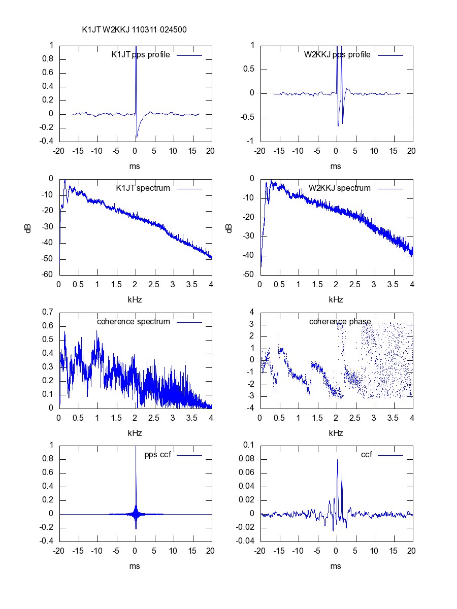
The plots, reading left to right from the top:
1. PPS pulse for station 1
- This is the result of folding the received data on itself with a 1 second offset, picking up the GPS-derived 1 pps signal and averaging out most of the other audio signal. (We also solve for the true sound card sampling rate.)
2. PPS pulse for station 2
- Same for the second receiving station. Note abnormal double pulse at W2KKJ. (A mystery thus far.)
3. Average spectrum at station 1
- Audio power spectrum of first station. The roll off may be due to the receiver passband or to the source spectrum. (Note that we are receiving an SSB signal using AM detectors, which will probably give low-frequency emphasis.)
4. Average spectrum at station 2
- Same for second receiving station.
5. Calibrated coherence spectrum (amplitude)
- Amplitude part of cross power spectrum of receiver 1 with receiver 2. Helps to show which part of analog spectrum shows a common signal at both receivers. If the receiving stations were listening to difference signals or widely different frequencies, the coherence only be noise.
6. Calibrated coherence spectrum (phase)
- Phase part of cross power spectrum. Those sections showing good signal to noise (up to about 2.2 kHz in this case) also indicate good coherence between receivers.
7. PPS cross correlation
- Cross-correlation between the 1pps signals at both stations. Has to be "perfect" because of analysis procedure.
8. W1AW cross correlation
- Cross-correlation, which is the Fourier transform of #5 and #6 above. In the case of simple propagation and good signal to noise, we expect a sharp peak at a time offset determined by the difference in time of arrival of the signal from W1AW. In this case we see multiple peaks, which could be partly instrumental (see plot #2) and partly because there are two propagation paths, e.g., single and double hop paths.
The easiest signals to work with are the time transmissions of WWV, WWVH, CHU, or other stations. These are naturally time-tagged at the source -- usually with a 1 pulse per second (1 pps) "tick". If your receiver also has a GPS-derived (or other) time marker, you can readily determine the propagation time between the transmitter and receiver.
To first order, the delay measurement can simply be made visually with an oscilloscope connected to the receiver's audio output signal with the sweep triggered by the GPS tick. However, you must also measure the RF input to AF output delay of the receiver, which can be some milliseconds.
Joe Taylor, K1JT, has developed a program called "wwv" that produces software delay solutions on a computer whose sound card input is connected to the receiver output. The program looks for a 1 pps signal from the GPS injected at the local receiver and also solves for one or more locations of the WWV (or WWVH) tick in the audio data. At times, it is possible to detect WWV at more than one delay, reflecting different propagation modes, such as 1 hop, 2 hop, etc. It is also possible to find WWVH and WWV simultaneously appearing at different delays.
The wwv software (for Windows) is available at http://www.physics.princeton.edu/pulsar/K1JT/wwv.exe with instructions at http://www.physics.princeton.edu/pulsar/K1JT/HFTOA_1.pdf.
Sample Results
The following graphs show WWV and WWVH data obtained at AA6E in Connecticut on Feb. 23-24, 2011 using the K1JT wwv program with data plotted in OpenOffice.org Spreadsheet.
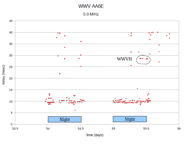
This plot shows all the delay solutions obtained over the run. (Note that the scattered points are invalid noise solutions. Good solutions fall in narrow delay ranges.) Usable signals are received only in the evenings, and WWVH makes an appearance toward morning of the second day.
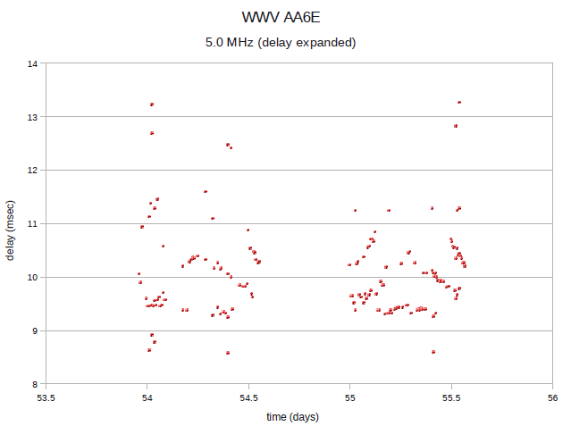
The second plot is the same data with the delay scale expanded to show information in the delays obtained from WWV. For each night, we seem to see 3 separate propagation modes, corresponding (perhaps) to 1, 2, and 3 hops between Colorado and Connecticut. [Added later: The separate delay curves may well indicate different reflection layers at different altitudes.] The delays are seen to increase as the ionosphere electron density lowers after sunset and to decrease in a symmetric fashion towards sunrise.
The complete data for this run (over all WWV frequencies) is available at http://groups.yahoo.com/group/hftoa/files/AA6E/aa6e_wwv_feb2324.pdf.